I sent my Open Drift modeling to a number of subject matter experts for expert review. I was very grateful for replies with constructive criticism from Sergei Prants (Head of Lab of Nonlinear Dynamical Systems, Head of Department of the Ocean and Atmosphere Physics Pacific Oceanological Institute of the Russian Academy of Sciences, David Griffin (CSIRO), Atsuhiko Isobe (Research Institute for Applied Mechanics, Kyushu Univ.) and Mike Eichorn.
One of the criticisms of my modeling was the Leeway drift coefficient I had calculated from my pool drift experiment used was far too high. I had used a Leeway drift coefficient of 0.07 but I was told normal leeway drift coefficients are typically 0.02 to maximum 0.04. I had measured a leeway drift coefficient of 0.02 for a mainly submerged but just floating object.
I realised from my pool experiment that I had measured the wind velocity at the surface of the water but the historical wind data I was using in the model was from 10m height so I needed to correct my measured wind speed to 10m height. This is because the wind speed slows down as it approaches the water surface.
In order to correct my measured velocity at about 10cm height to 10m height I needed to know the “roughness distance” of the water. This is the theoretical distance above the surface that the wind velocity reduces to zero. Roughly speaking, smooth water like in the pool experiment has a roughness distance of 0.1mm. Choppy water has a roughness distance of 1-10mm and extremely rough seas might have a roughness distance of 10-50mm.
To convert wind velocity at height X to 10m you use the formula: –  .
.
However I realised this was just guessing the roughness distance which could vary results dramatically. I needed a way to measure the roughness distance whilst performing the measurement. This could be done by using two data logging anemometers recording at two different heights at the same time. I purchased 2 x UT363BT Mini Anemometer’s with Bluetooth and used one old iPhone and my iPhone to log the data from each.
I built a jig to hold each anemometer at exactly 2m separation, then measured the distance from bottom anemometer to surface.
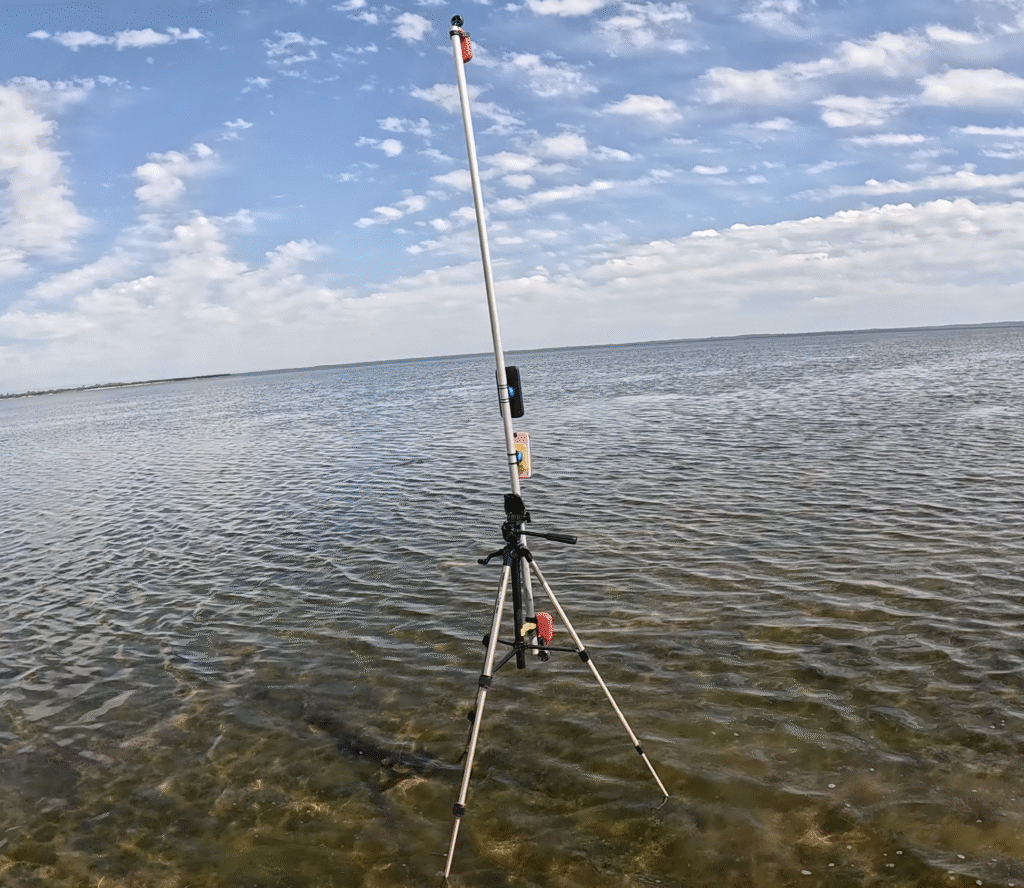
To test results worked I logged the wind for a few minutes at one height, and then again at a different height on water and then on grass. The results for both roughness distance and 10m wind velocity should be the same independent of the distance above surface.
***Add results here
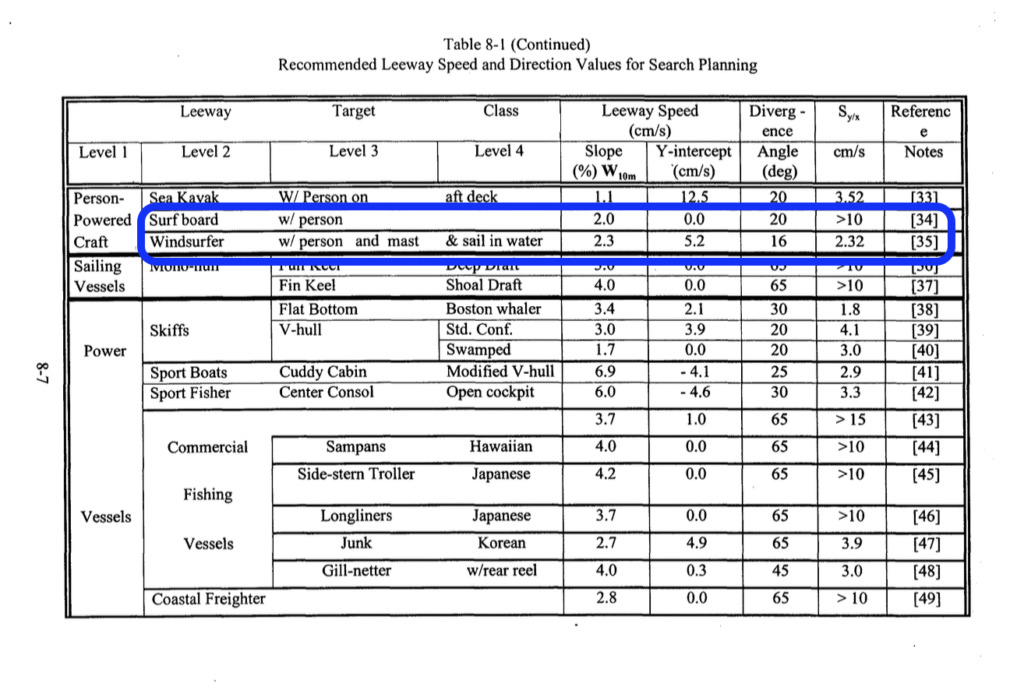
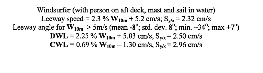
Many of the professional debris drift experts refer to a landmark 1999 study by the US coast guard that can be found here. This was an extensive study on drifting objects for the purpose of search and rescue. This paper in turn references a 1960 study by Chapline W.E. as the source of the Leeway drift coefficient for a surfboard. This brief study is included as an Appendix D in the US coast guard document. In it they reference a surfboard as the object most like aircraft debris. This surfboard was experimentally determined to have a Leeway drift coefficient of 0.02 which was far below my experimentally obtained result even accounting for adjustment to 10m wind height.
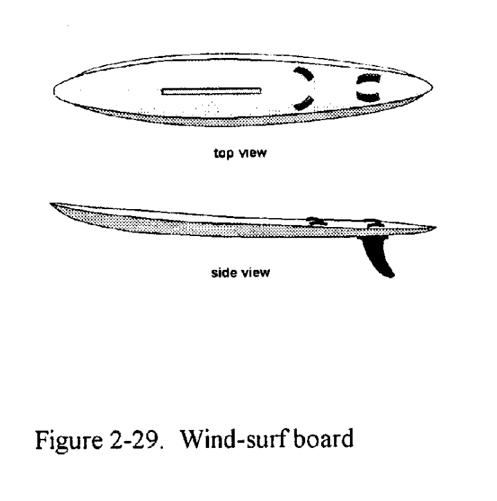
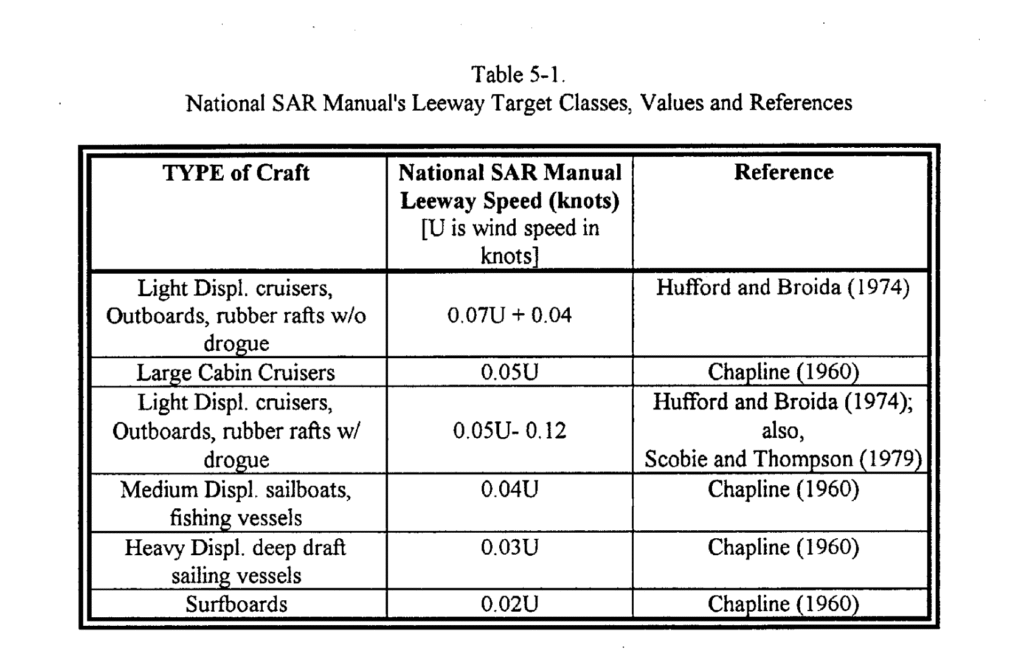
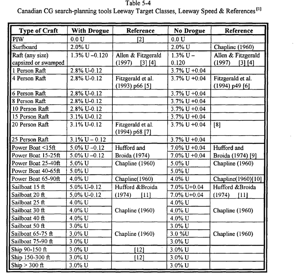
This 0.02 Leeway drift coefficient also felt wrong as I was an active windsurfer and I knew that if I let go of my board, the board would be swept away faster than I could swim. I read further and I was surprised to find that the “surfboard” was actually a windsurf board but with both the sail in the water and a person on board…i.e. a windsurfer in distress. This was nothing like a lightweight piece of aircraft composite honeycomb.
The pool experiment was definitely not real world but I knew so good places to do more experimentation that had no water currents or waves that were also shallow so easy to perform experiments. This was the estuary south of Perth called the Mandurah estuary. Much of the first 500m from land around the estuary is about knee height water, has only a tiny inlet and outlet to the sea so not affected by ocean waves. This I knew for certain as if the wind dropped to zero whilst windsurfing, the water surface would turn to glass within a few seconds. Tidal effects are minimal relative to the wind velocity.
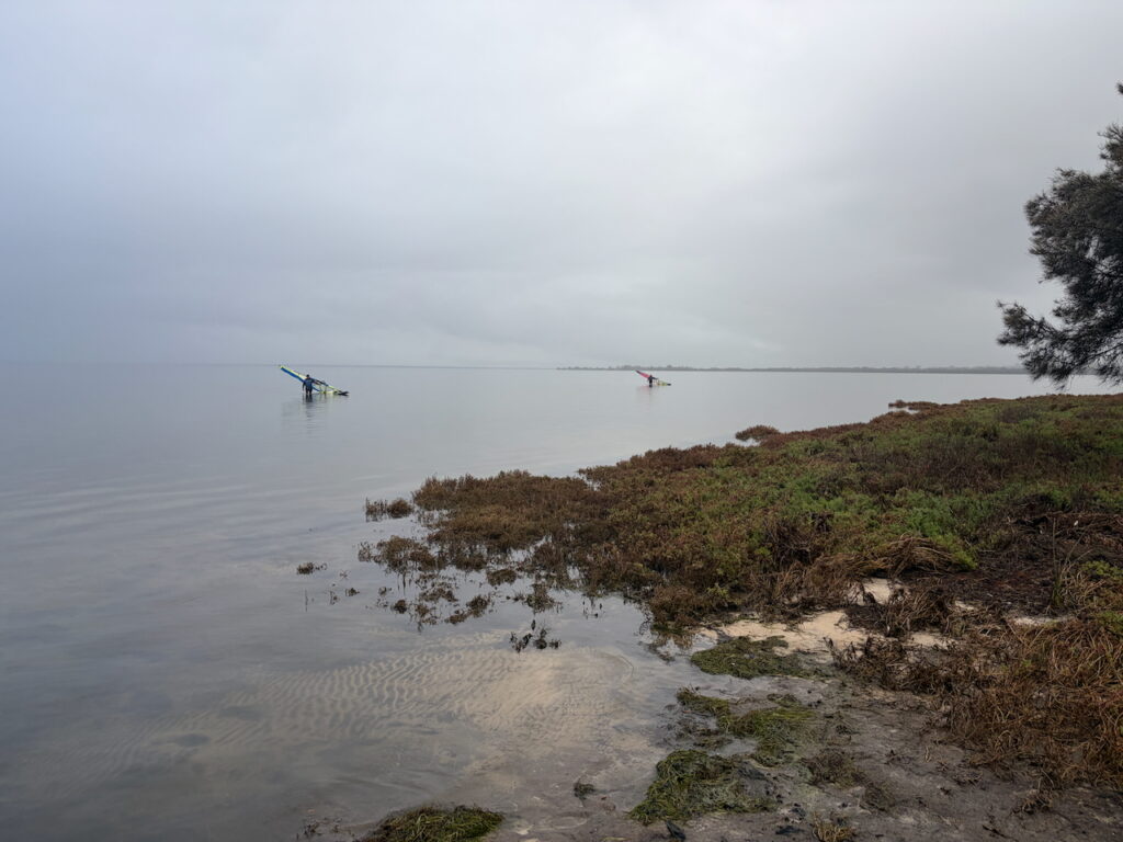
The first test I performed before I had obtained the anemometers. I used two wind surf boards without fins, both with extremely accurate doppler GPS units mounted on them. These GPS units are certified units we use for GPSTeamChallenge which is a World wide Windsurf race. I used two boards as one was extremely modern (just a few months old with little use) and the other was quite old so I assumed (wrongly) that the density of each would be different. However, the density of the new and older board turned out to be almost identical. older iSonic 97litre 6.8Kg: density 0.07g/cm^3, brand new Tribal88, 6.1kg: density = 0.069 g/cm^3.
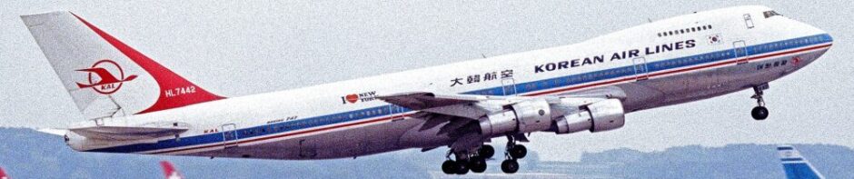
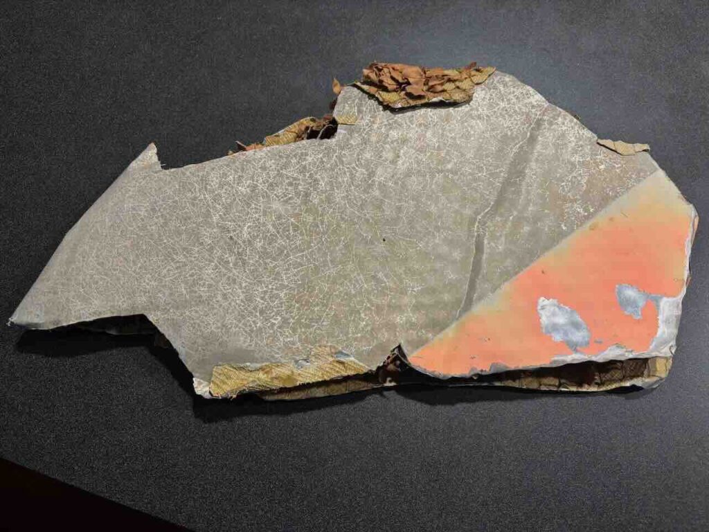
I also placed a real piece of KAL007 debris in the water at the same time. This had a density of 0.0892 g/cm^3. I measured the density by photographing the debris, importing the image into Fusion 360 (a CAD program), calibrating the image, drawing a spline around the edge, extruding it exactly 1 1/4″ then obtaining the volume. I weighed the debris at 159grams.
I walked beside the debris but a few meters away with a similar GPS as placing a GPS on the debris would unfairly increase the debris density. The GPS unit weighs 149grams, almost doubling the mass of debris.
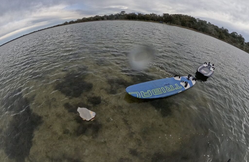
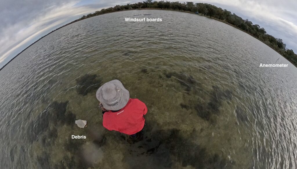
The windsurf boards both travelled at the same speed but significantly faster than the debris. However, I noticed the debris felt a lot heavier when I retrieved it and sure enough it had been taking on water. So I dried the debris out and decided to 3D print the same shape and size. I adjusted the infil density so the weight was exactly the same as the real wreckage. Then I raced the real wreckage vs the 3D print.
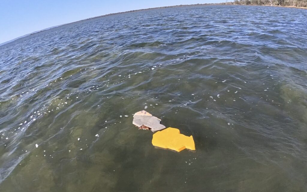
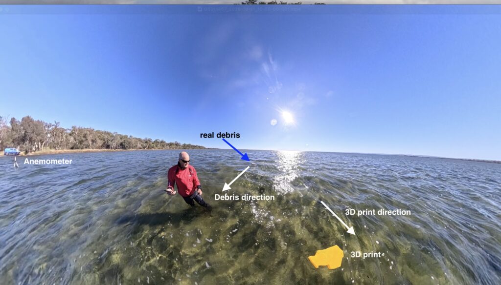
The 3D print travelled as expected much faster than the real debris due to the real debris slowly sinking. However, despite being the same orientation at the start, not only was the 3D print much further ahead but it was also travelling at a completely different angle off the wind. Why was that? I wasn’t aware at the time but the 3D print maintained the original orientation but the real wreckage had gybed. It’s not clear in this photo but zooming in one can see this is the case.
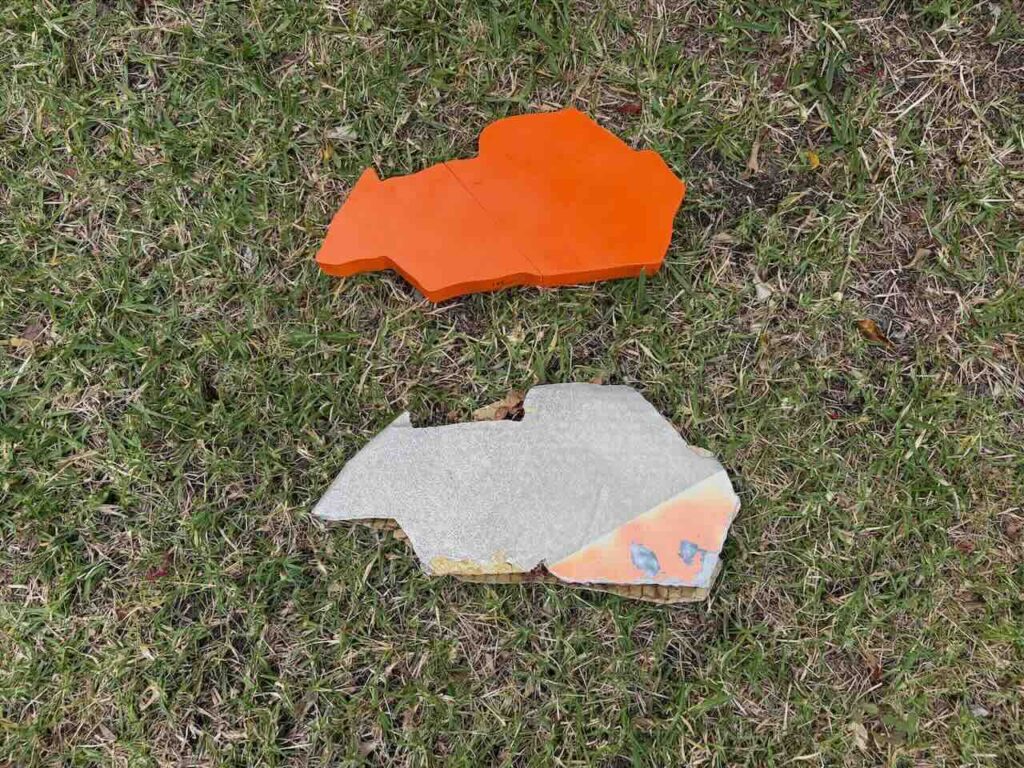
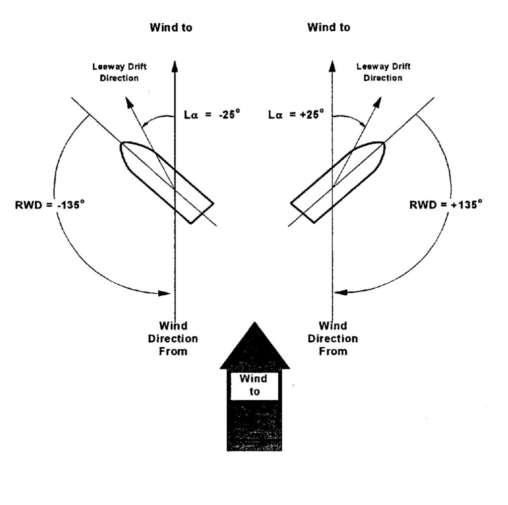
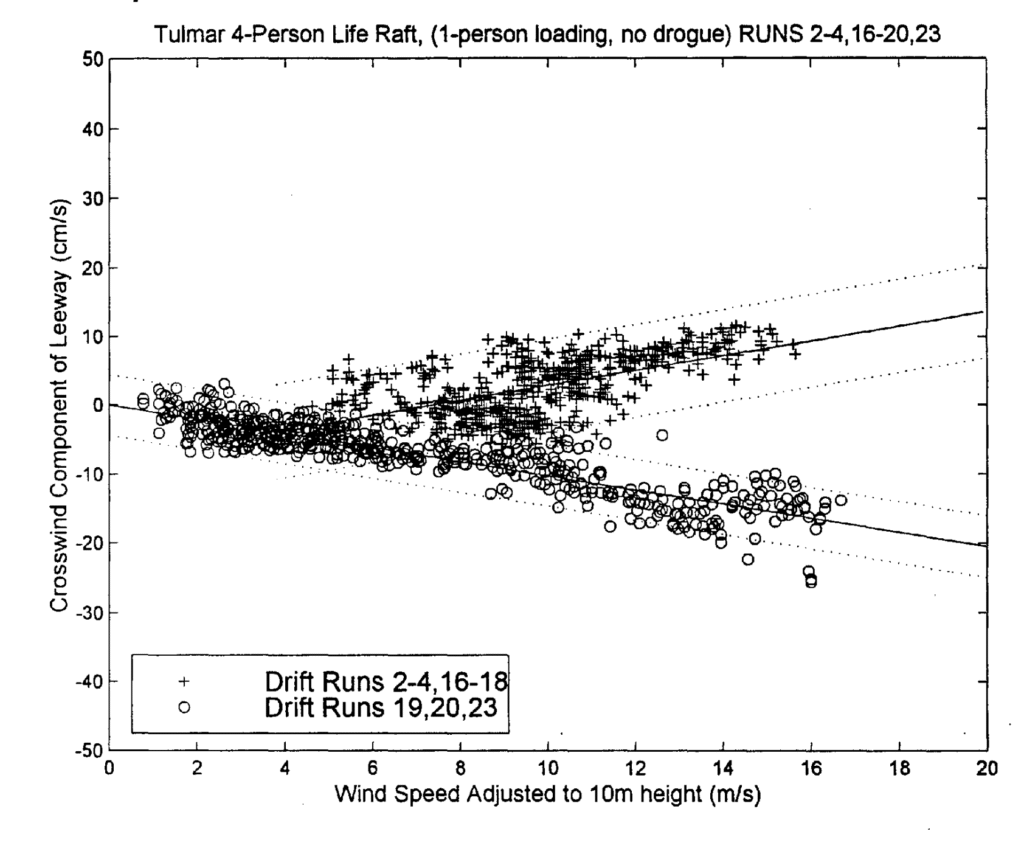
This was starting to get interesting so I read the US Coast Guard paper in full and learnt that most objects drifting exhibit what is known as “Tack Locking” and Bifurcation. That is they get “locked” at a certain orientation and then travel at a certain angle +/- off the wind but not directly downwind. With a keeled craft like a yacht this angle is up to 65 deg away from the direction of the wind.
This was interesting so I printed another identical piece of wreckage then repeated the experiments in a moderate breeze (6m/s). However, the pieces kept gybing (spinning 180 deg around the vertical axis) so I could not get any manful results.
I tried again but the wind was even higher (8m/S) and the 3D prints were both gybing and now flipping…i.e. they were getting lifted by the wind and flipped about the horizontal axis perpendicular to the wind so again no consistent measure of any bifurcation.
I decided on a statistical approach so printed 45 identical pieces of wreckage in as random shape as I could imagine. These pieces were small costing only a few cents each. The idea was to launch all at once and they should cluster into two distinct clumps.
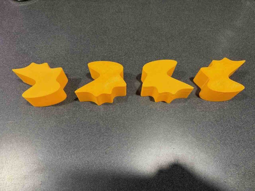
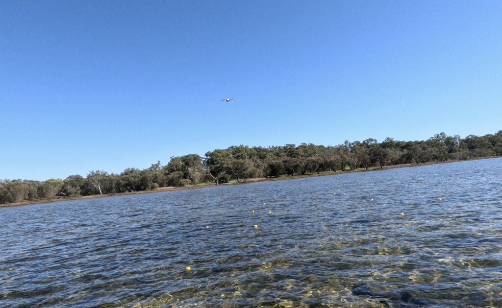
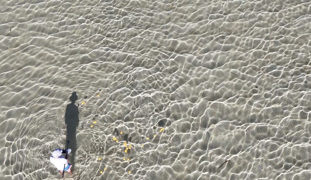
Now these crazy ducks were certainly going off in different directions but instead of 2 directions they were clearly going in 4 different directions. Once they beached they were in 4 main distinct clumps. There were also some laggards, 3D prints that were leaking and taking on water. Interestingly they went slower but at a much larger angle off the wind. I tried to capture using a drone but other than the initial launch the small size meant they were very difficult to see in the bright conditions.
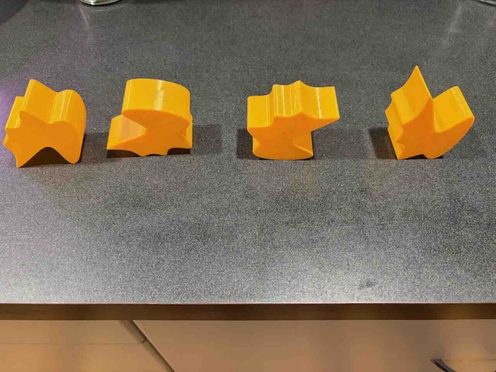
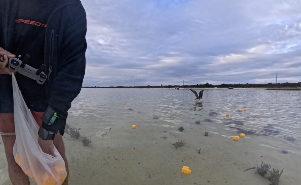
I then realised that these crazy ducks always aligned or “tack locked” in one of 4 orientations so exhibited quadrification. I also realised the actual wreckage also would take on any 4 possible orientations and also travel at 4 distinct angles off the wind. The angles they travelled seemed to be some function of the chirality or asymmetry of the debris about the center of mass. The larger prints were also much easier to see with the drone so I printed each piece of wreckage 4 times and repeated the experiment.
In light winds below 4 m/s the debris almost always maintained the same orientation as launch. However as the wind speed increased the waves generated by the wind increased the probability they would gybe. It was interesting that a gybe now inverted the drift angle off the wind but also changed from an inner to outer track or visa versa.
As wind increased further at approximately 8m/s as well as gybing the debris would now get lifted by the wind and “flipped” in the horizontal plane perpendicular to the wind. If the objects flipped they would maintain a similar but different angle off the wind. i.e. instead of inverting the angle and changing the track, they would just jump from inner to outer tack or visa versa. However, this flipping man they were now travelling faster than just drifting as the object ‘jumped’ at least its width along the wind. As the wind increased to 10m/s the debris started flying. Thus instead of a constant Leeway drift coefficient the debris exhibits an exponential Leeway drift coefficient. Some images better describe what is occurring.
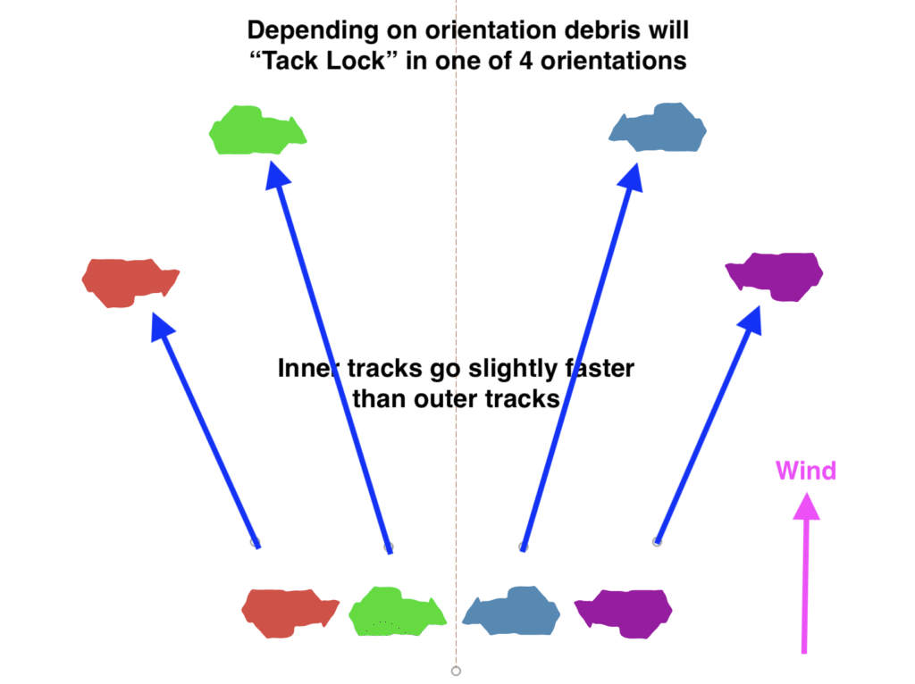
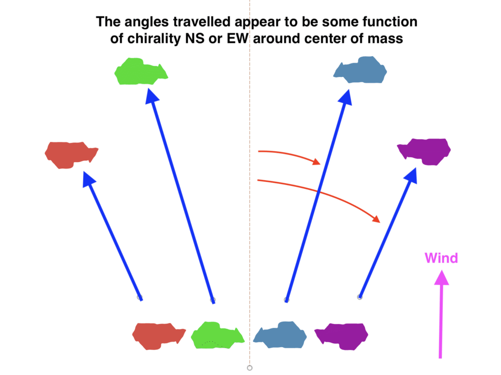
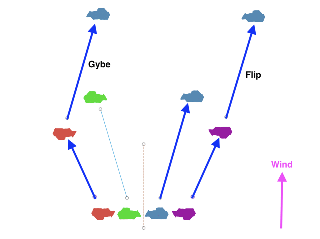
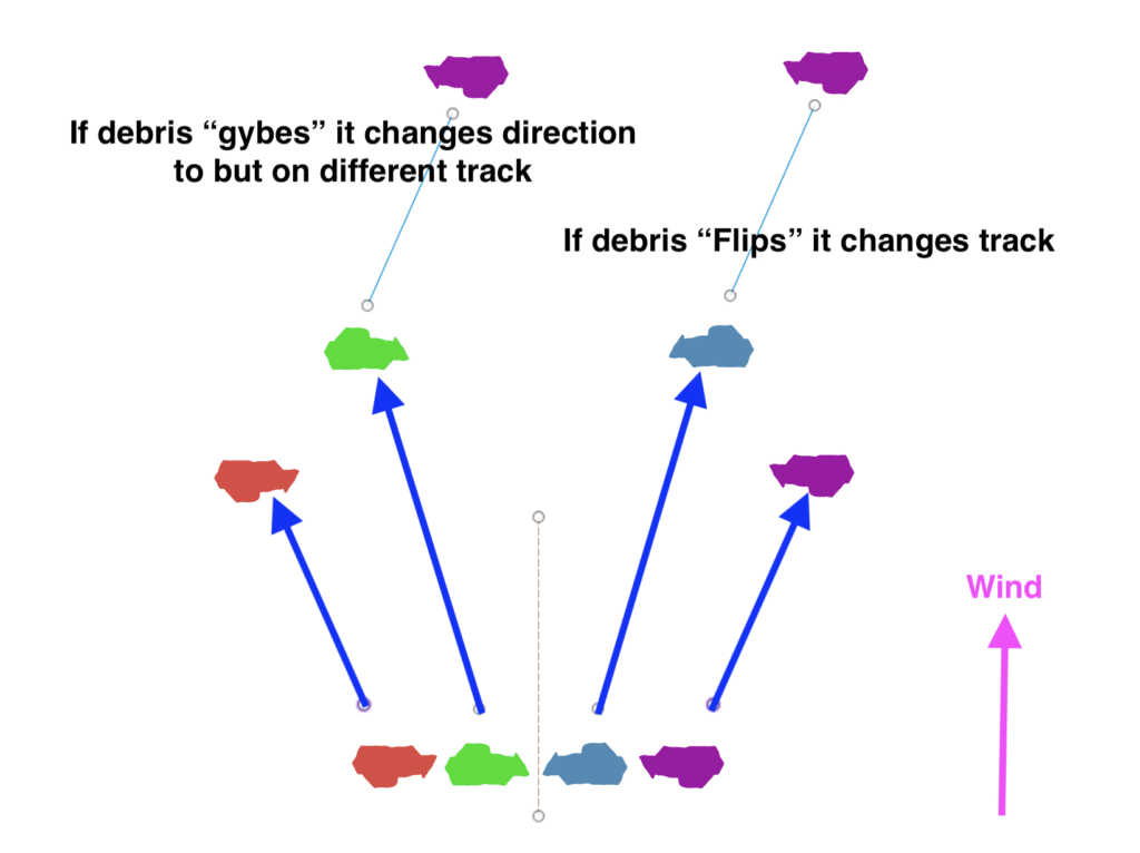
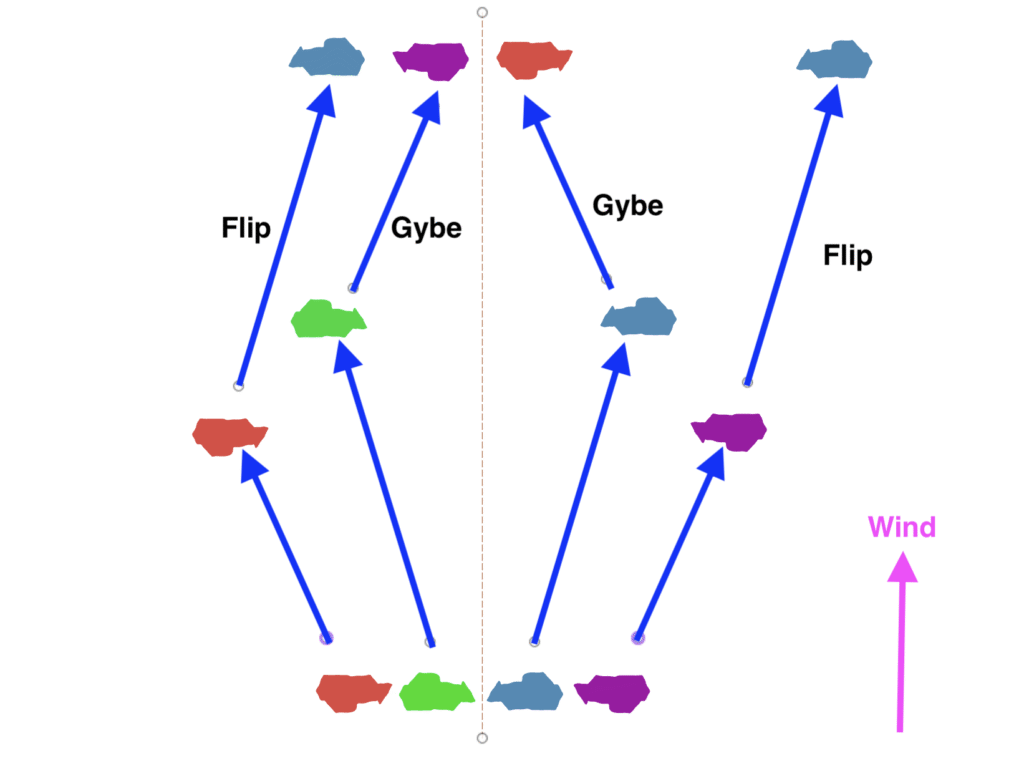
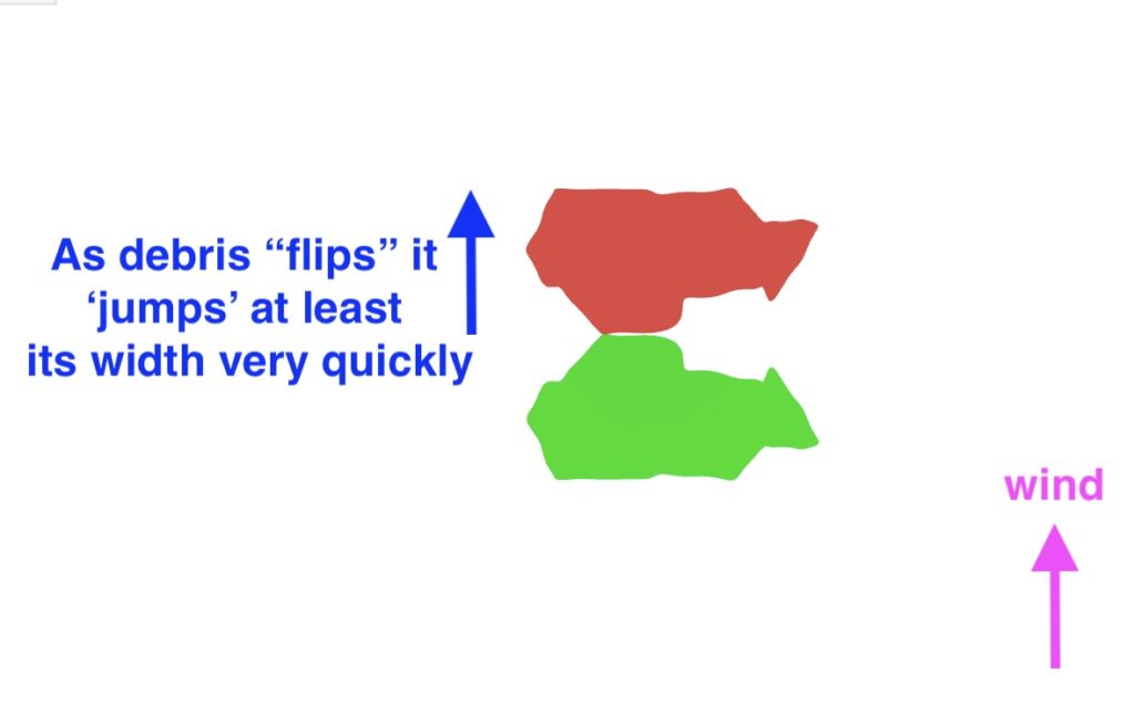
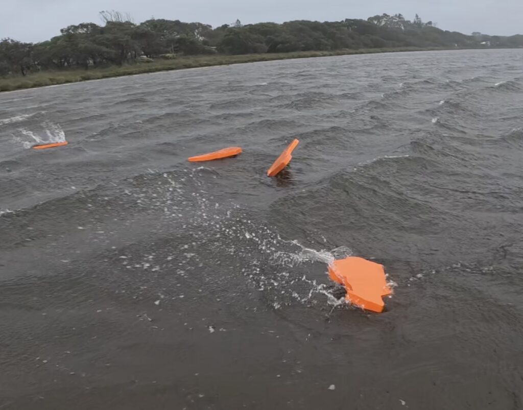
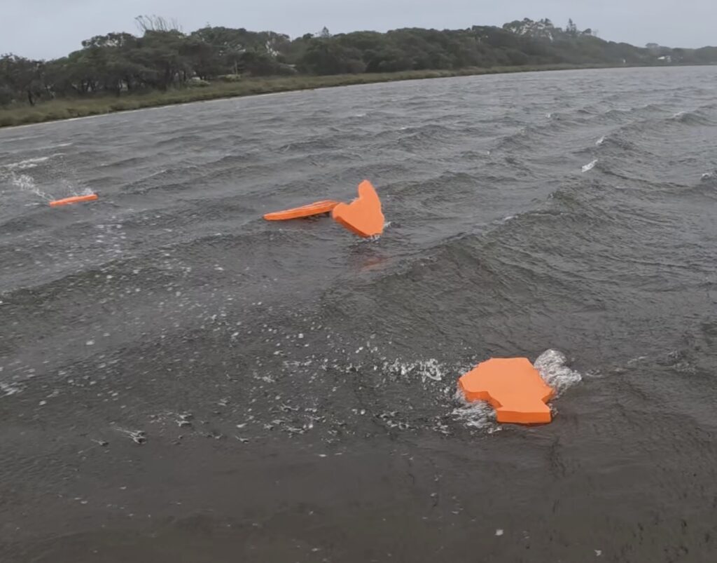
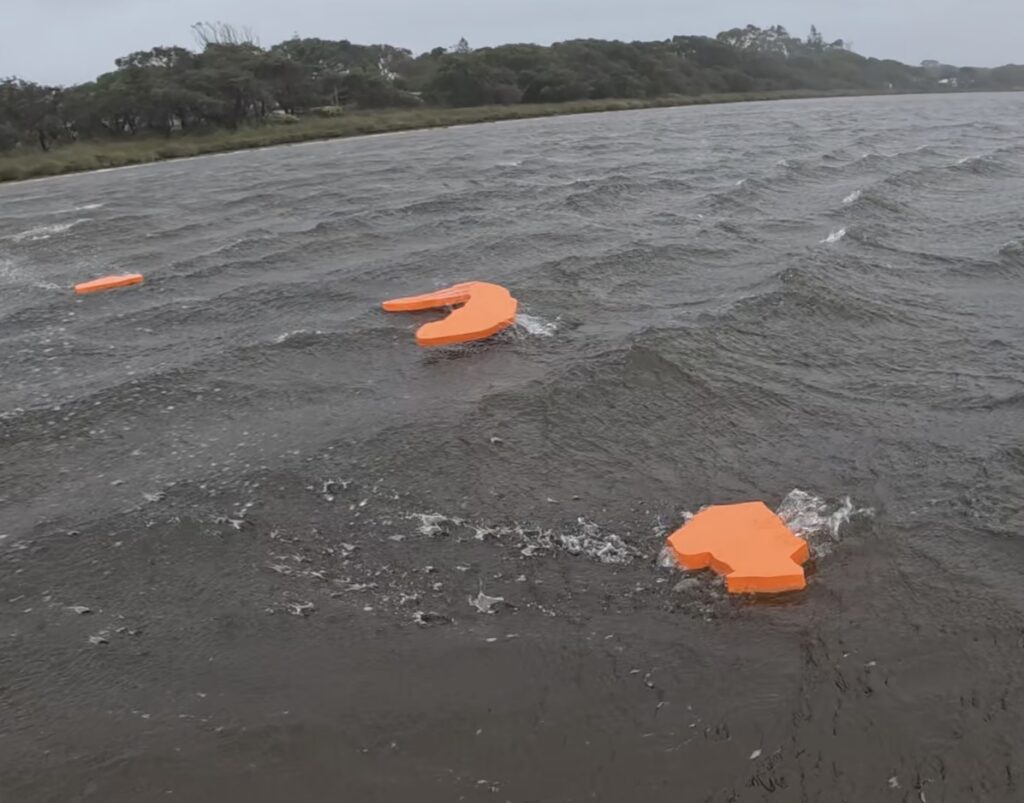
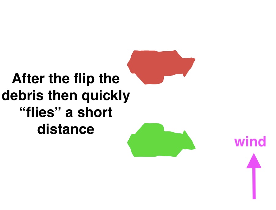
So for light winds, debris would spread quite quickly as each piece tack locked. However in increasing winds the gybing and flipping would tend to reduce the spread and the debris would tend to approach the wind direction…i.e. Leeway angle would approach 0.
A brief video of some of the experimentation here
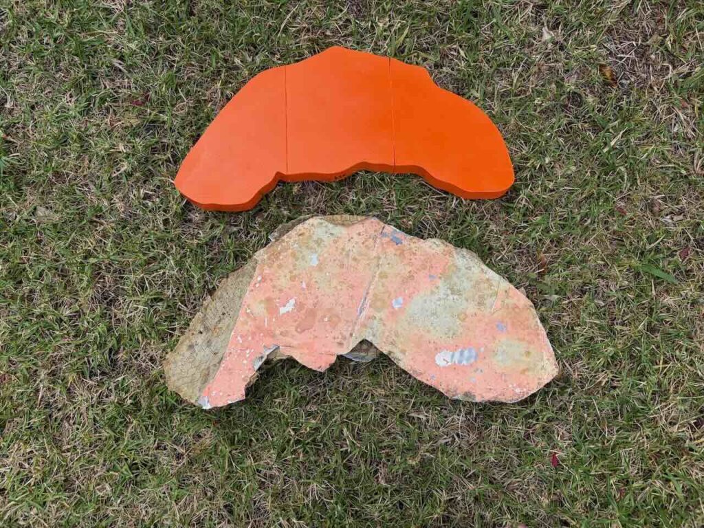
Since the other piece of wreckage I had found was curved I 3D printed a replica of it. I somehow managed to get the scale wrong but the density was the same. The main difference in behaviour of this debris over the flat was that it gybed far easier. Therefore its leeway drift coefficient would be expected to be close to zero.
Since I had two pieces of actual wreckage and many photos of other wreckage I started to wonder what the minimum and maximum Leeway drift angles could be. It seemed a reasonable mathematical concept that all the wreckage shapes could possibly be reduced to a basic rectangular shape with a diagonal cutout of dimension X. The rectangle measured 300m x 213mm. 213 = 300/sqrt(2) I initially printed 4 pieces with X =150mm with the same density as the real wreckage.
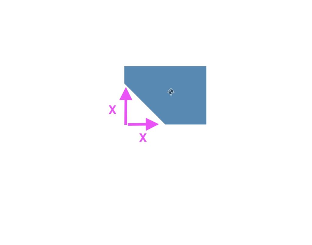
The challenge was to find some kind of mathematical method to predict how the objects would travel depending on the value X. I asked numerous AI models to come up with a prediction. Claude and Gemini said the problem was impossible. Grok figured that the difference in CG (Center of Gravity) to center of bounding box was the clue. A bounding box is the smallest piece of rectangular material required to machine any shape. As X is increased from 0, the bounding box center remains fixed but the CG drifts away from the cutout side. Grok did correctly predict the basic angle each would take but was wildly wrong with the magnitude of the angle. It over estimated the angle significantly. Grok correctly predicted that the direction of the CG relative to center of bounding box would determine the basic direction travelled. i.e.; if the CG was on the left of the center of bounding box it would in general travel left. However, it incorrectly calculated whether the debris would take the inside or outside track depending whether the cutout faced the wind or was leeward.
Up until this point I was only using one anemometer to measure the wind speed. The second one I purchased later and only just arrived as this point. So I started repeating the Leeway drift coefficient experiment but this time measuring the wind speed at two different heights. Unfortunately the winds in my area have been very light so as I write this only a small subset of the winds required have been measured. For wind speed of 4.79m/s Leeway = 0.041, 5.6m/S = 0.045. At 9.4m/s the leeway coefficient is 0.057
For the area of interest during the time of interest in sept 1983 the wind conditions were quite strong. Many days between 10-20m/s. The maximum wind so far I’ve experimented in is 10m/s.
| Date | Min (m/s) | Max (m/s) | Mean (m/s) |
| 1 Sep | 0.0 | 6.8 | 2.4 |
| 2 Sep | 0.1 | 11.5 | 4.1 |
| 3 Sep | 0.1 | 11.5 | 5.1 |
| 4 Sep | 0.0 | 9.6 | 4.2 |
| 5 Sep | 0.0 | 9.0 | 3.5 |
| 6 Sep | 0.0 | 12.7 | 4.7 |
| 7 Sep | 0.0 | 13.5 | 6.3 |
| 8 Sep | 0.0 | 14.4 | 6.8 |
| 9 Sep | 0.0 | 14.8 | 5.3 |
| 10 Sep | 0.0 | 12.9 | 4.8 |
| 11 Sep | 0.0 | 17.2 | 6.6 |
| 12 Sep | 0.2 | 19.7 | 9.2 |
| 13 Sep | 0.1 | 14.5 | 7.9 |
| 14 Sep | 0.0 | 14.0 | 4.9 |
| 15 Sep | 0.1 | 14.8 | 6.5 |
| 16 Sep | 0.0 | 15.6 | 6.7 |
Even at 10m/s wind the debris exhibits quite a lot of flipping, flying and gybing. With an average of 10.1m/s the Leeway coefficient corrected to 10m height has already increased to 0.058. I fully expect wind speeds above 10m/s to exhibit much higher Leeway drift coefficient.
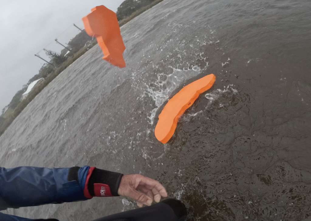
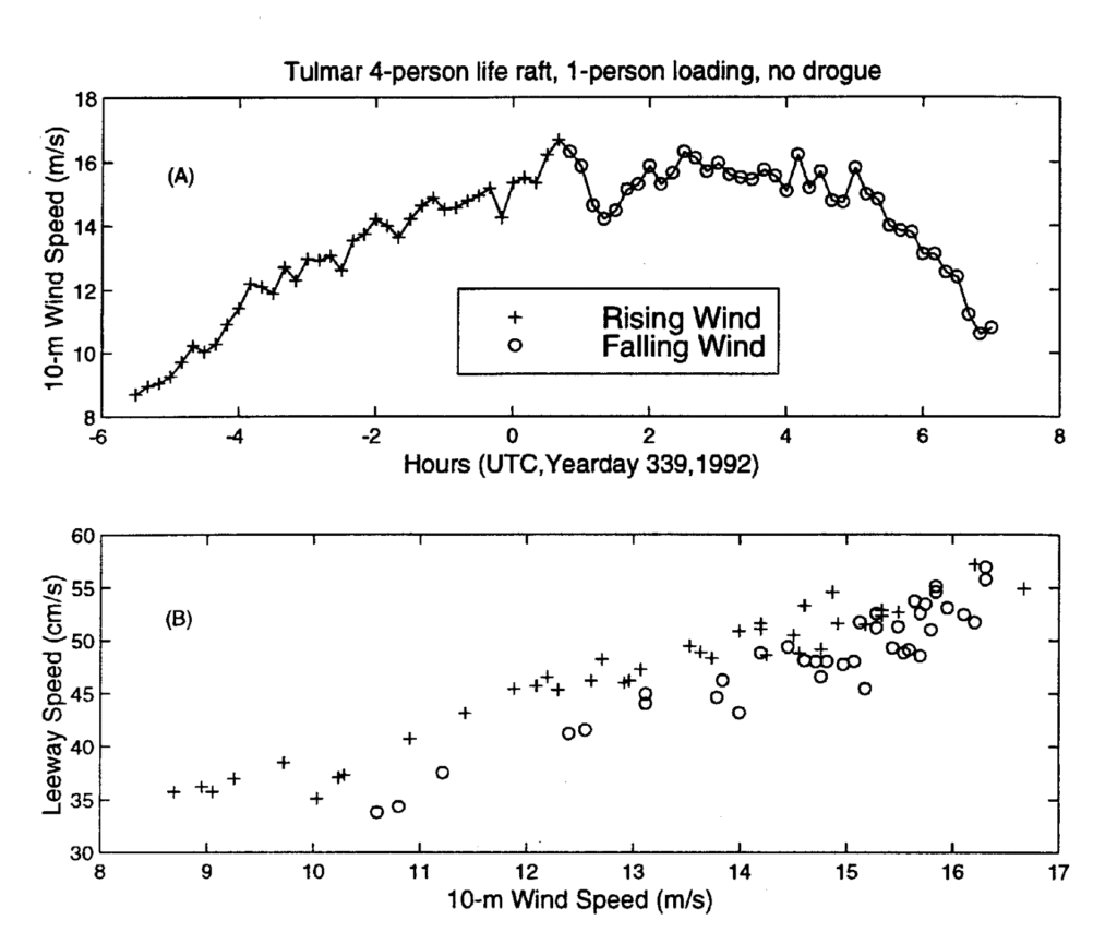
To further complicate Leeway drift calculations the US Coast Guard study showed that the Leeway drift coefficient changes whether the wind is rising or falling. In a rising wind the Leeway is higher than on a falling wind. Quote:”This behavior may be associated with the more effective transfer of energy from the atmosphere to the oceans during rising wind conditions than during decreasing wind conditions. When waves are growing, the atmosphere is transferring energy into the sea surface; when waves are decreasing, the waves are transferring energy back to the atmosphere.