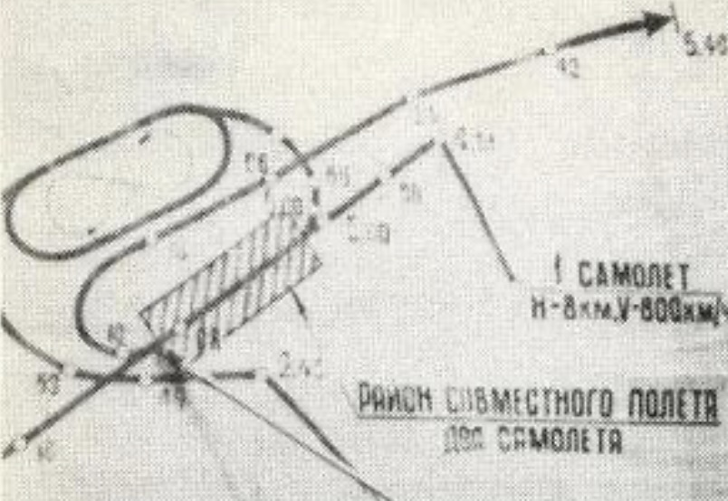
In the 1993 ICAO report, two radar plots provided by the Russians are included. They are Chart 12 and Chart 13 on page 48 and 50 respectively. In addition another radar chart of KAL-007’s rendezvous with a RC-135 was presented by Ogarkov on Sept 9, 1983. These radar plots are shown below.
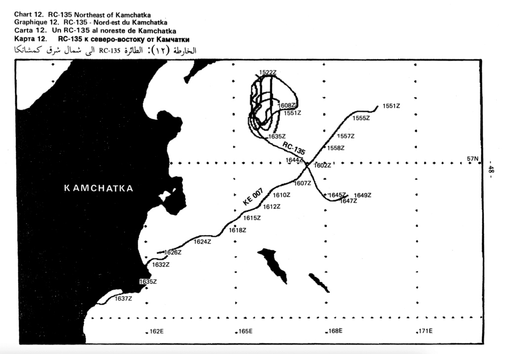
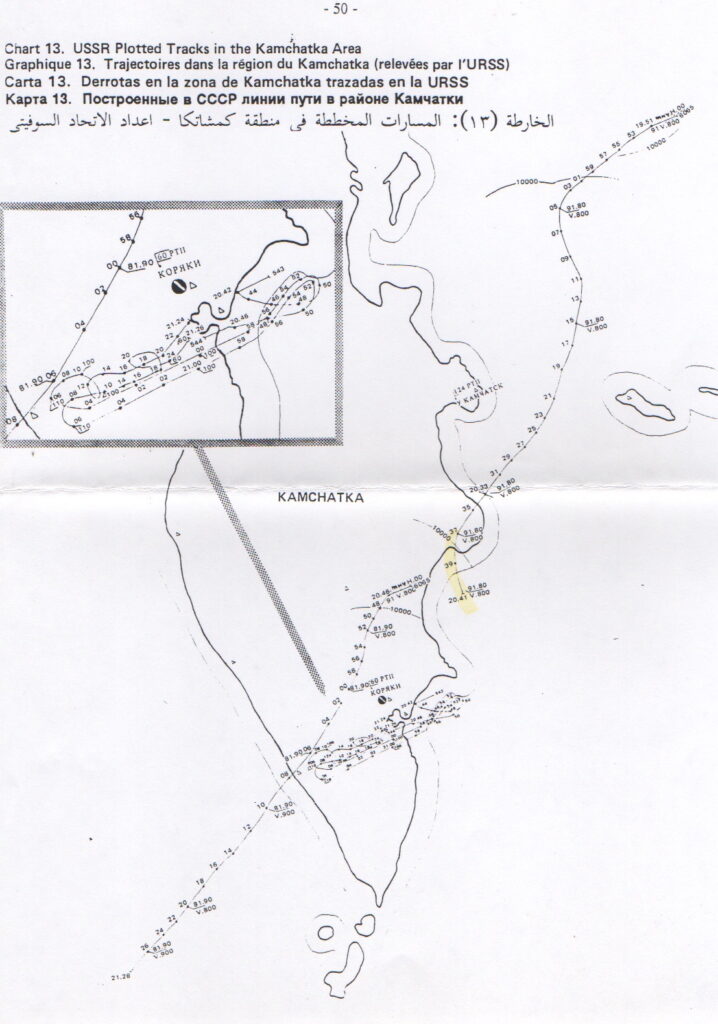
ICAO curiously makes no mention of the fact that both these radar tracks reportedly to be of KAL-007 don’t follow a constant magnetic heading as is their conclusion to how the flight went off course. Both tracks clearly show multiple turns. A casual examination makes it appear both radar traces are of KAL007, however there is much more information in these radar traces that the Soviets wanted to show but also appear to align with a single intruder story of the US.
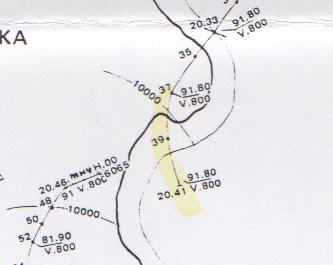
The Soviets also made the maps confusing by using different times for each map. Chart 12 uses UTC, Chart 13 Moscow time and Ogarkov uses local Kamchatka time.
On chart 13 it is clear that the aircraft is both slowing down and speeding up from the spacing of the time stamps. Again these are not actions of an innocent stray airliner.
Importing and Georeferencing both maps in Mapwarper.net and over laying them show that the paths are completely separate in both space and time showing that at least two aircraft overflew Kamchatka. It is clear that chart 12 was the aircraft that made the rendezvous with the RC-135 or other aircraft.
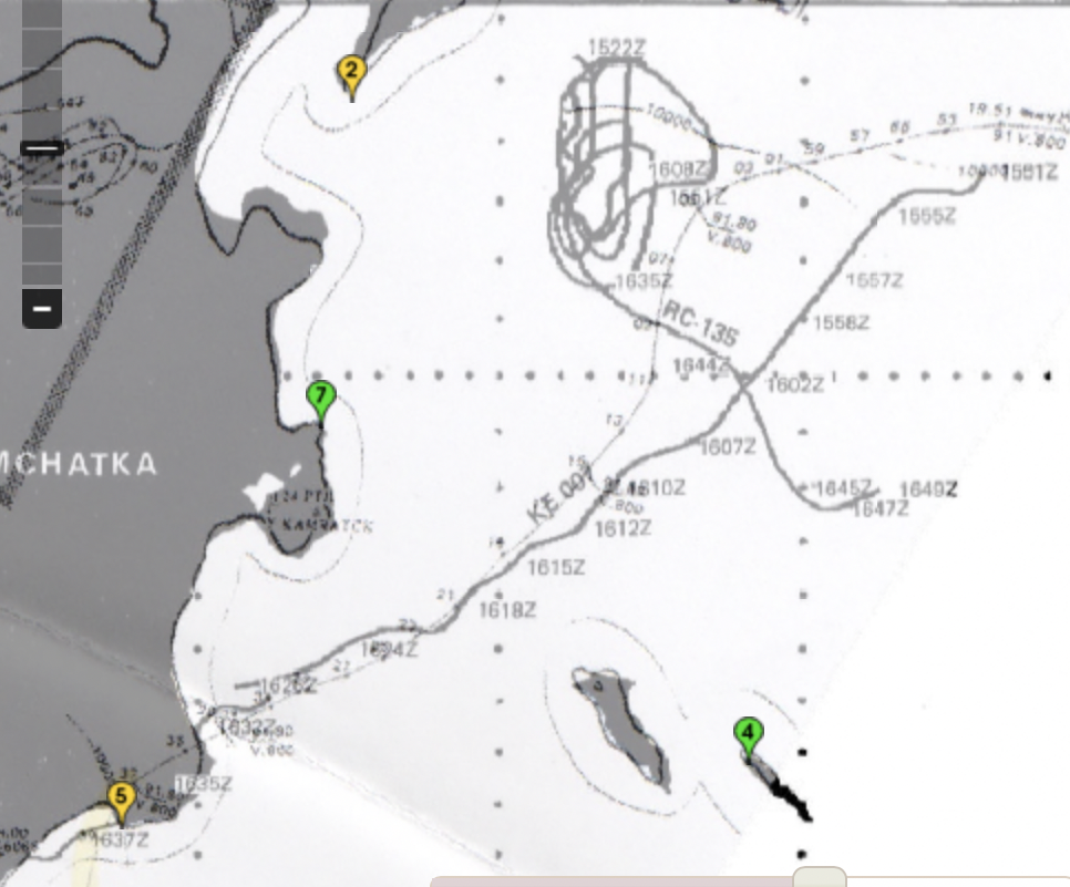
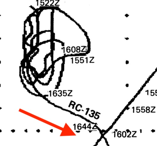
Whilst the Ogarkov map has no land masses to allow georeferencing it is clear that the rendezvous show by Ogakov is completely different to that of chart 12. In chart 12 the RC-135 radar trace leaves the pattern at 16:35UTC and crosses 007’s trace at 90 deg about 42 min later and is exiting its holding pattern in a SE direction. Ogarkov’s map shows the RC-135 travelling with 007 for 10 minutes then exiting the pattern in a NE direction a few minutes earlier at 16:26-16:28.
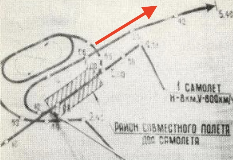
This suggests there were two aircraft flying the figure 8’s and one flew for 10 minutes with the pings from the radar traces overlaid. This appears to be a mid air refuelling.
The Georeferenced maps can be loaded into QGIS and the coordinates extracted for the radar traces. Since they are clearly labelled with times the velocity of the aircraft can be determined. The coordinates and speeds for each trace can be found for chart 12 here and chart 13 here.
It is beneficial to visualise traces together in an animation. Note in this animation the KE-007 path is unknown but a plausible path is shown based on known timing. Intruder #1 is the trace from Chart 13 and Intruder #2 is the trace from chart 12.
For chart 13 the speeds are as low as 280knots and as high as 880knots. These speeds are not possible for an 747 flying at 33,000ft. Chart 12 is harder to extract exact coordinates but speeds calculated range from 1100knts to 300knots, again not possible for a 747. These speeds are also not possible for a RC-135 but more like those of a EF-1111. If neither of these traces were from a 747, where was KAL007?
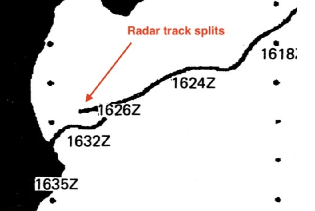
On both chart 12 and 13 the radar traces split. One trace on chart 12 seems to stop at 16:26Z and a different track emerges with the next time shown at 16:32Z. On chart 13 one radar trace appears to head south and be lost and another trace starts at 20:46. This may be one aircraft being lost on radar or two aircraft.